Information to lightning-fast JAX

Hey there, fellow Python fanatic! Have you ever ever wished your NumPy code run at supersonic velocity? Meet JAX!. Your new greatest pal in your machine studying, deep studying, and numerical computing journey. Consider it as NumPy with superpowers. It might probably mechanically deal with gradients, compile your code to run quick utilizing JIT, and even run on GPU and TPU with out breaking a sweat. Whether or not you’re constructing neural networks, crunching scientific knowledge, tweaking transformer fashions, or simply attempting to hurry up your calculations, JAX has your again. Let’s dive in and see what makes JAX so particular.

This information gives an in depth introduction to JAX and its ecosystem.

Studying Goals

• Clarify JAX’s core rules and the way they differ from Numpy.
• Apply JAX’s three key transformations to optimize Python code. Convert NumPy operations into environment friendly JAX implementation.
• Determine and repair widespread efficiency bottlenecks in JAX code. Implement JIT compilation appropriately whereas avoiding typical Pitfalls.
• Construct and prepare a Neural Community from scratch utilizing JAX. Implement widespread machine studying operations utilizing JAX’s useful strategy.
• Resolve optimization issues utilizing JAX’s computerized differentiation. Carry out environment friendly matrix operations and numerical computations.
• Apply efficient debugging methods for JAX-specific points. Implement memory-efficient patterns for large-scale computations.

This text was revealed as part of the Knowledge Science Blogathon.

What’s JAX?

In accordance with the official documentation, JAX is a Python library for acceleration-oriented array computation and program transformation, designed for high-performance numerical computing and large-scale machine studying. So, JAX is actually NumPy on steroids, It combines acquainted NumPy-style operations with computerized differentiation and {hardware} acceleration. Consider it as getting the perfect of three worlds.

• NumPy’s elegant syntax and array operation
• PyTorch like computerized differentiation functionality
• XLA’s (Accelerated Linear Algebra) for {hardware} acceleration and compilation advantages.

Why does JAX Stand Out?

What units JAX aside is its transformations. These are highly effective features that may modify your Python code:

• JIT: Simply-In-Time compilation for quicker execution
• Grad: Automated differentiation for computing gradients
• vmap: Mechanically vectorization for batch processing

Here’s a fast look:

import jax.numpy as jnp
from jax import grad, jit
# Outline a easy operate
@jit  # Velocity it up with compilation
def square_sum(x):
    return jnp.sum(jnp.sq.(x))
# Get its gradient operate mechanically
gradient_fn = grad(square_sum)
# Strive it out
x = jnp.array([1.0, 2.0, 3.0])
print(f"Gradient: {gradient_fn(x)}")

Output:

Gradient: [2. 4. 6.]

Getting Began with JAX

Under we’ll observe some steps to get began with JAX.

Step1: Set up

Organising JAX is simple for CPU-only use. You should use the JAX documentation for extra info.

Step2: Creating Setting for Undertaking

Create a conda surroundings in your venture

# Create a conda env for jax
$ conda create --name jaxdev python=3.11

#activate the env
$ conda activate jaxdev

# create a venture dir title jax101
$ mkdir jax101

# Go into the dir
$cd jax101

Step3: Putting in JAX

Putting in JAX within the newly created surroundings

# For CPU solely
pip set up --upgrade pip
pip set up --upgrade "jax"

# for GPU
pip set up --upgrade pip
pip set up --upgrade "jax[cuda12]"

Now you might be able to dive into actual issues. Earlier than getting your palms soiled on sensible coding let’s study some new ideas. I can be explaining the ideas first after which we’ll code collectively to know the sensible viewpoint.

First, get some motivation, By the way in which, why will we study a brand new library once more? I’ll reply that query all through this information in a step-by-step method so simple as attainable. 

Why Study JAX?

Consider JAX as an influence instrument. Whereas NumPy is sort of a dependable hand noticed, JAX is sort of a fashionable electrical noticed. It requires a bit extra steps and data, however the efficiency advantages are value it for intensive computation duties.

• Efficiency: Jax code can run considerably quicker than Pure Python or NumPy code, particularly on GPU and TPUs
• Flexibility: It’s not only for machine learning- JAX excels in scientific computing, optimization, and simulation.
• Trendy Method: JAX encourages useful programming patterns that result in cleaner, extra maintainable code.

Within the subsequent part, we’ll dive deep into JAX’s transformation, beginning with the JIT compilation. These transformations are what give JAX its superpowers, and understanding them is vital to leveraging JAX successfully.

Important JAX Transformations

JAX’s transformations are what really set it other than the numerical computation libraries akin to NumPy or SciPy. Let’s discover every one and see how they’ll supercharge your code.

JIT or Simply-In-Time Compilation

Simply-in-time compilation optimizes code execution by compiling components of a program at runtime moderately than forward of time.

How JIT works in JAX?

In JAX, jax.jit transforms a Python operate right into a JIT-compiled model. Adorning a operate with @jax.jit captures its execution graph, optimizes it, and compiles it utilizing XLA. The compiled model then executes, delivering vital speedups, particularly for repeated operate calls.

Right here is how one can attempt it.

import jax.numpy as jnp
from jax import jit
import time


# A computationally intensive operate
def slow_function(x):
    for _ in vary(1000):
        x = jnp.sin(x) + jnp.cos(x)
    return x


# The identical operate with JIT
@jit
def fast_function(x):
    for _ in vary(1000):
        x = jnp.sin(x) + jnp.cos(x)
    return x

Right here is similar operate, one is only a plain Python compilation course of and the opposite one is used as a JAX’s JIT compilation course of. It would calculate the 1000 knowledge factors sum of sine and cosine features. we’ll evaluate the efficiency utilizing time.

# Evaluate efficiency
x = jnp.arange(1000)

# Heat-up JIT
fast_function(x)  # First name compiles the operate

# Time comparability
begin = time.time()
slow_result = slow_function(x)
print(f"With out JIT: {time.time() - begin:.4f} seconds")

begin = time.time()
fast_result = fast_function(x)
print(f"With JIT: {time.time() - begin:.4f} seconds")

The end result will astonish you. The JIT compilation is 333 occasions quicker than the traditional compilation. It’s like evaluating a bicycle with a Buggati Chiron.

Output:

With out JIT: 0.0330 seconds
With JIT: 0.0010 seconds

JIT may give you a superfast execution enhance however you should use it correctly in any other case will probably be like driving Bugatti on a muddy village highway that gives no supercar facility.

Widespread JIT Pitfalls

JIT works greatest with static shapes and kinds. Keep away from utilizing Python loops and situations that rely upon array values. JIT doesn’t work with the dynamic arrays.

# Dangerous - makes use of Python management circulate
@jit
def bad_function(x):
    if x[0] > 0:  # This would possibly not work effectively with JIT
        return x
    return -x


# print(bad_function(jnp.array([1, 2, 3])))


# Good - makes use of JAX management circulate
@jit
def good_function(x):
    return jnp.the place(x[0] > 0, x, -x)  # JAX-native situation


print(good_function(jnp.array([1, 2, 3])))

Output:

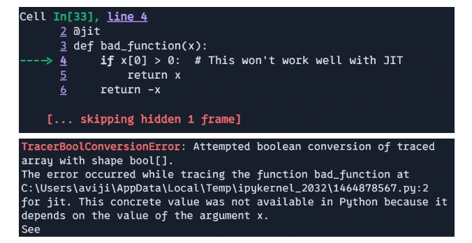
Meaning bad_function is unhealthy as a result of JIT was not positioned within the worth of x throughout calculation.

Output:

[1 2 3]

Limitations and Concerns

• Compilation Overhead: The primary time a JIT-compiled operate is executed, there may be some overhead attributable to compilation. The compilation value might outweigh the efficiency advantages for small features or these referred to as solely as soon as.
• Dynamic Python Options: JAX’s JIT requires features to be “static”. Dynamic management circulate, like altering shapes or values based mostly on Python loops, isn’t supported within the compiled code. JAX supplied options like `jax.lax.cond` and `jax.lax.scan` to deal with dynamic management circulate.

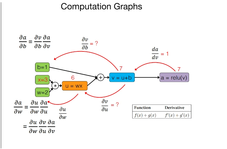
Automated Differentiation

Automated differentiation, or autodiff, is a computation method for calculating the by-product of features precisely and successfully. It performs a vital position in optimizing machine studying fashions, particularly in coaching neural networks, the place gradients are used to replace mannequin parameters.

How does Automated differentiation work in JAX?

Autodiff works by making use of the chain rule of calculus to decompose complicated features into easier ones, calculating the by-product of those sub-functions, after which combining the outcomes. It data every operation in the course of the operate execution to assemble a computational graph, which is then used to compute derivatives mechanically.

There are two important modes of auto-diff:

• Ahead Mode: Computes derivatives in a single ahead cross by way of the computational graph, environment friendly for features with a small variety of parameters.
• Reverse Mode: Computes derivatives in a single backward cross by way of the computational graph, environment friendly for features with a lot of parameters.

Key options in JAX computerized differentiation

• Gradient Computation(jax.grad): `jax.grad` computes the by-product of a scaler-output operate for its enter. For features with a number of inputs, a partial by-product will be obtained.
• Increased-Order By-product(jax.jacobian, jax.hessian) :   JAX helps the computation of higher-order derivatives, akin to Jacobians and Hessains, making it appropriate for superior optimization and physics simulation.
• Composability with different JAX Transformation:   Autodiff in JAX integrates seamlessly with different transformations like `jax.jit` and `jax.vmap` permitting for environment friendly and scalable computation.
• Reverse-Mode Differentiation(Backpropagation):   JAX’s auto-diff makes use of reverse-mode differentiation for scaler-output features, which is very efficient for deep studying duties.

import jax.numpy as jnp
from jax import grad, value_and_grad


# Outline a easy neural community layer
def layer(params, x):
    weight, bias = params
    return jnp.dot(x, weight) + bias


# Outline a scalar-valued loss operate
def loss_fn(params, x):
    output = layer(params, x)
    return jnp.sum(output)  # Lowering to a scalar


# Get each the output and gradient
layer_grad = grad(loss_fn, argnums=0)  # Gradient with respect to params
layer_value_and_grad = value_and_grad(loss_fn, argnums=0)  # Each worth and gradient

# Instance utilization
key = jax.random.PRNGKey(0)
x = jax.random.regular(key, (3, 4))
weight = jax.random.regular(key, (4, 2))
bias = jax.random.regular(key, (2,))

# Compute gradients
grads = layer_grad((weight, bias), x)
output, grads = layer_value_and_grad((weight, bias), x)

# A number of derivatives are simple
twice_grad = grad(grad(jnp.sin))
x = jnp.array(2.0)
print(f"Second by-product of sin at x=2: {twice_grad(x)}")

Output:

Second derivatives of sin at x=2: -0.9092974066734314

Effectiveness in JAX

• Effectivity:  JAX’s computerized differentiation is very environment friendly attributable to its integration with XLA, permitting for optimization on the machine code degree.
• Composability:  The power to mix totally different transformations makes JAX a robust instrument for constructing complicated machine studying pipelines and Neural Networks structure akin to CNN, RNN, and Transformers.
• Ease of Use: JAX’s syntax for autodiff is easy and intuitive, enabling customers to compute gradient with out delving into the small print of XLA and complicated library APIs.

JAX Vectorize Mapping

In JAX, `vmap` is a robust operate that mechanically vectorizes computations, permitting you to use a operate over batches of information with out manually writing loops. It maps a operate over an array axis (or a number of axes) and evaluates it effectively in parallel, which may result in vital efficiency enhancements.

How vmap Works in JAX?

The vmap operate automates the method of making use of a operate to every ingredient alongside a specified axis of an enter array whereas preserving the effectivity of the computation. It transforms the given operate to just accept batched inputs and execute the computation in a vectorized method.

As an alternative of utilizing specific loops, vmap permits operations to be carried out in parallel by vectorizing over an enter axis. This leverages the {hardware}’s functionality to carry out SIMD (Single Instruction, A number of Knowledge) operations, which can lead to substantial speed-ups.

Key Options of vmap

• Automated Vectorization:   vamp automates the batching of computations, making it easy to parallel code over batch dimensions with out altering the unique operate logic.
• Composability with different Transformations:    It really works seamlessly with different JAX transformations, akin to jax.grad for differentiation and jax.jit for Simply-In-Time compilation, permitting for extremely optimized and versatile code.
• Dealing with A number of Batch Dimensions:   vmap helps mapping over a number of enter arrays or axes, making it versatile for numerous use circumstances like processing multi-dimensional knowledge or a number of variables concurrently.

import jax.numpy as jnp
from jax import vmap


# A operate that works on single inputs
def single_input_fn(x):
    return jnp.sin(x) + jnp.cos(x)


# Vectorize it to work on batches
batch_fn = vmap(single_input_fn)

# Evaluate efficiency
x = jnp.arange(1000)

# With out vmap (utilizing a listing comprehension)
result1 = jnp.array([single_input_fn(xi) for xi in x])

# With vmap
result2 = batch_fn(x)  # A lot quicker!


# Vectorizing a number of arguments
def two_input_fn(x, y):
    return x * jnp.sin(y)


# Vectorize over each inputs
vectorized_fn = vmap(two_input_fn, in_axes=(0, 0))

# Or vectorize over simply the primary enter
partially_vectorized_fn = vmap(two_input_fn, in_axes=(0, None))


# print
print(result1.form)
print(result2.form)
print(partially_vectorized_fn(x, y).form)

Output:

(1000,)
(1000,)
(1000,3)

Effectiveness of vmap in JAX

• Efficiency Enhancements: By vectorizing computations, vmap can considerably velocity up execution by leveraging parallel processing capabilities of recent {hardware} like GPUs, and TPUs(Tensor processing items).
• Cleaner Code: It permits for extra concise and readable code by eliminating the necessity for handbook loops.
• Compatibility with JAX and Autodiff: vmap will be mixed with computerized differentiation (jax.grad), permitting for the environment friendly computation of derivatives over batches of information.

When to Use Every Transformation

Utilizing @jit when:

• Your operate is named a number of occasions with related enter shapes.
• The operate comprises heavy numerical computations.

Use grad when:

• You want derivatives for optimization.
• Implementing machine studying algorithms
• Fixing differential equations for simulations

Use vmap when:

• Processing batches of information with.
• Parallelizing computations
• Avoiding specific loops

Matrix Operations and Linear Algebra Utilizing JAX

JAX gives complete assist for matrix operations and linear algebra, making it appropriate for scientific computing, machine studying, and numerical optimization duties. JAX’s linear algebra capabilities are just like these present in libraries like NumPY however with further options akin to computerized differentiation and Simply-In-Time compilation for optimized efficiency.

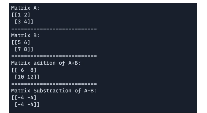
Matrix Addition and Subtraction

These operation are carried out element-wise matrices of the identical form.

# 1 Matrix Addition and Subtraction:

import jax.numpy as jnp

A = jnp.array([[1, 2], [3, 4]])
B = jnp.array([[5, 6], [7, 8]])

# Matrix addition
C = A + B
# Matrix subtraction
D = A - B

print(f"Matrix A: n{A}")
print("===========================")
print(f"Matrix B: n{B}")
print("===========================")
print(f"Matrix adition of A+B: n{C}")
print("===========================")
print(f"Matrix Substraction of A-B: n{D}")

Output:

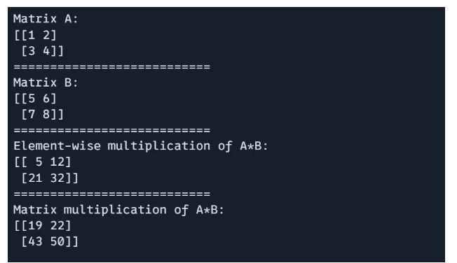
Matrix Multiplication

JAX assist each element-wise multiplication and dor product-based matrix multiplication.

# Aspect-wise multiplication
E = A * B

# Matrix multiplication (dot product)
F = jnp.dot(A, B)

print(f"Matrix A: n{A}")
print("===========================")
print(f"Matrix B: n{B}")
print("===========================")
print(f"Aspect-wise multiplication of A*B: n{E}")
print("===========================")
print(f"Matrix multiplication of A*B: n{F}")

Output:

Matrix Transpose

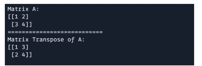
The transpose of a matrix will be obtained utilizing `jnp.transpose()`

# Matric Transpose
G = jnp.transpose(A)

print(f"Matrix A: n{A}")
print("===========================")
print(f"Matrix Transpose of A: n{G}")

Output:

Matrix Inverse

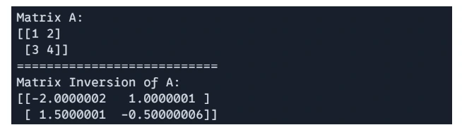
JAX gives operate for matrix inversion utilizing `jnp.linalg.inv()`

# Matric Inversion
H = jnp.linalg.inv(A)

print(f"Matrix A: n{A}")
print("===========================")
print(f"Matrix Inversion of A: n{H}")

Output:

Matrix Determinant

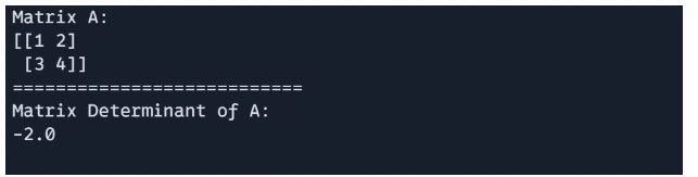
Determinant of a matrix will be calculate utilizing `jnp.linalg.det()`.

# matrix determinant
det_A = jnp.linalg.det(A)

print(f"Matrix A: n{A}")
print("===========================")
print(f"Matrix Determinant of A: n{det_A}")

Output:

Matrix Eigenvalues and Eigenvectors

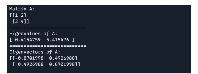
You may compute the eigenvalues and eigenvectors of a matrix utilizing `jnp.linalg.eigh()`

# Eigenvalues and Eigenvectors
import jax.numpy as jnp

A = jnp.array([[1, 2], [3, 4]])
eigenvalues, eigenvectors = jnp.linalg.eigh(A)

print(f"Matrix A: n{A}")
print("===========================")
print(f"Eigenvalues of A: n{eigenvalues}")
print("===========================")
print(f"Eigenvectors of A: n{eigenvectors}")

Output:

Matrix Singular Worth Decomposition

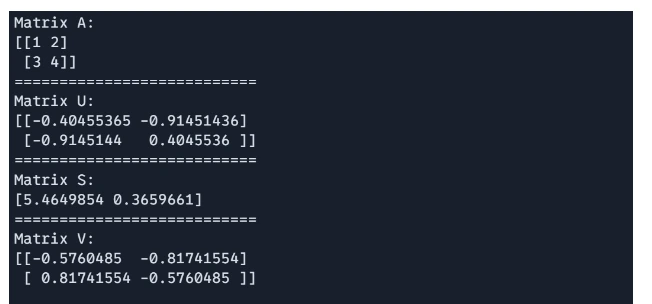
SVD is supported by way of `jnp.linalg.svd`, helpful in dimensionality discount and matrix factorization.

# Singular Worth Decomposition(SVD)

import jax.numpy as jnp

A = jnp.array([[1, 2], [3, 4]])
U, S, V = jnp.linalg.svd(A)

print(f"Matrix A: n{A}")
print("===========================")
print(f"Matrix U: n{U}")
print("===========================")
print(f"Matrix S: n{S}")
print("===========================")
print(f"Matrix V: n{V}")

Output:

Fixing System of Linear Equations

To resolve a system of linear equation Ax = b, we use `jnp.linalg.resolve()`, the place A is a sq. matrix and b is a vector or matrix of the identical variety of rows.

# Fixing system of linear equations
import jax.numpy as jnp

A = jnp.array([[2.0, 1.0], [1.0, 3.0]])
b = jnp.array([5.0, 6.0])
x = jnp.linalg.resolve(A, b)

print(f"Worth of x: {x}")

Output:

Worth of x: [1.8 1.4]

Computing the Gradient of a Matrix Perform

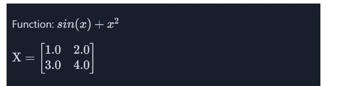
Utilizing JAX’s computerized differentiation, you possibly can compute the gradient of a scalar operate with respect to a matrix.
We’ll calculate gradient of the beneath operate and values of X

Perform

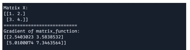
# Computing the Gradient of a Matrix Perform
import jax
import jax.numpy as jnp


def matrix_function(x):
    return jnp.sum(jnp.sin(x) + x**2)


# Compute the grad of the operate
grad_f = jax.grad(matrix_function)

X = jnp.array([[1.0, 2.0], [3.0, 4.0]])
gradient = grad_f(X)

print(f"Matrix X: n{X}")
print("===========================")
print(f"Gradient of matrix_function: n{gradient}")

Output:

These most helpful operate of JAX utilized in numerical computing, machine studying, and physics calculation. There are lots of extra left so that you can discover.

Scientific Computing with JAX

JAX’s highly effective libraries for scientific computing, JAX is greatest for scientific computing for its advance options akin to JIT compilation, computerized differentiation, vectorization, parallelization, and GPU-TPU acceleration. JAX’s capacity to assist excessive efficiency computing makes it appropriate for a variety of scientific purposes, together with physics simulations, machine studying, optimization and numerical evaluation.

We’ll discover an Optimization Downside on this part.

Optimization Issues

Allow us to undergo the optimization issues steps beneath:

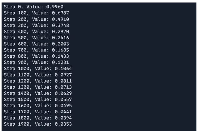
Step1: Outline the operate to reduce(or the issue)

# Outline a operate to reduce (e.g., Rosenbrock operate)

@jit

def rosenbrock(x):

    return sum(100.0 * (x[1:] - x[:-1] ** 2.0) ** 2.0 + (1 - x[:-1]) ** 2.0)

Right here, the Rosenbrock operate is outlined, which is a standard take a look at drawback in optimization. The operate takes an array x as enter and computes a valie that represents how far x is from the operate’s world minimal. The @jit decorator is used to allow Jut-In-Time compilation, which velocity up the computation by compiling the operate to run effectively on CPUs and GPUs.

Step2: Gradient Descent Step Implementation

# Gradient descent optimization

@jit

def gradient_descent_step(x, learning_rate):

    return x - learning_rate * grad(rosenbrock)(x)

This operate performs a single step of the gradient descent optimization. The gradient of the Rosenbrock operate is calculated utilizing grad(rosenbrock)(x), which gives the by-product with respects to x. The brand new worth of x is up to date by subtraction the gradient scaled by a learning_rate.The @jit is doing the identical as earlier than.

Step3: Operating the Optimization Loop

# Optimize
x = jnp.array([0.0, 0.0])  # Place to begin

learning_rate = 0.001

for i in vary(2000):

    x = gradient_descent_step(x, learning_rate)

    if i % 100 == 0:

        print(f"Step {i}, Worth: {rosenbrock(x):.4f}")

The optimization loop initializes the start line x and performs 1000 iterations of gradient descent. In every iteration, the gradient_descent_step operate updates based mostly on the present gradient. Each 100 steps, the present step quantity and the worth of the Rosenbrock operate at x are printed, offering the progress of the optimization.

Output:

Fixing Actual-world physics drawback with JAX

We’ll simulate a bodily system the movement of a damped harmonic oscillator, which fashions issues like a mass-spring system with friction, shock absorbers in automobiles, or oscillation in electrical circuits. Is it not good? Let’s do it.

Step1: Parameters Definition

import jax
import jax.numpy as jnp


# Outline parameters
mass = 1.0  # Mass of the item (kg)
damping = 0.1  # Damping coefficient (kg/s)
spring_constant = 1.0  # Spring fixed (N/m)

# Outline time step and whole time
dt = 0.01  # Time step (s)
num_steps = 3000  # Variety of steps

The mass, damping coefficient, and spring fixed are outlined. These decide the bodily properties of the damped harmonic oscillator.

Step2: ODE Definition

# Outline the system of ODEs
def damped_harmonic_oscillator(state, t):
    """Compute the derivatives for a damped harmonic oscillator.

    state: array containing place and velocity [x, v]
    t: time (not used on this autonomous system)
    """
    x, v = state
    dxdt = v
    dvdt = -damping / mass * v - spring_constant / mass * x
    return jnp.array([dxdt, dvdt])

  The damped harmonic oscillator operate defines the derivatives of the place and velocity of the oscillator, representing the dynamical system.

Step3: Euler’s Methodology

# Resolve the ODE utilizing Euler's technique
def euler_step(state, t, dt):
    """Carry out one step of Euler's technique."""
    derivatives = damped_harmonic_oscillator(state, t)
    return state + derivatives * dt

A easy numerical technique is used to resolve the ODE. It approximates the state on the subsequent time step on the premise of the present state and by-product.

Step4: Time Evolution Loops

# Preliminary state: [position, velocity]
initial_state = jnp.array([1.0, 0.0])  # Begin with the mass at x=1, v=0

# Time evolution
states = [initial_state]
time = 0.0
for step in vary(num_steps):
    next_state = euler_step(states[-1], time, dt)
    states.append(next_state)
    time += dt

# Convert the record of states to a JAX array for evaluation
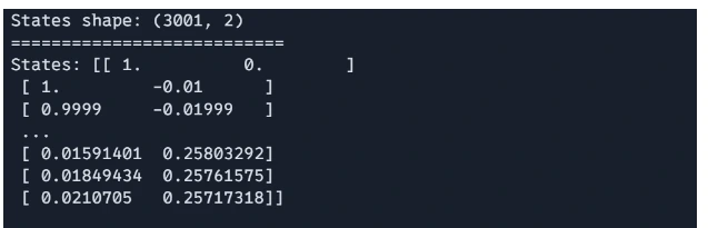
states = jnp.stack(states)

The loop iterates by way of the desired variety of time steps, updating the state at every step utilizing Euler’s technique.

Output:

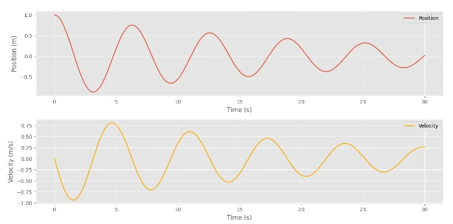
Step5: Plotting The Outcomes

Lastly, we are able to plot the outcomes to visualise the habits of the damped harmonic oscillator.

# Plotting the outcomes
import matplotlib.pyplot as plt

plt.model.use("ggplot")

positions = states[:, 0]
velocities = states[:, 1]
time_points = jnp.arange(0, (num_steps + 1) * dt, dt)

plt.determine(figsize=(12, 6))
plt.subplot(2, 1, 1)
plt.plot(time_points, positions, label="Place")
plt.xlabel("Time (s)")
plt.ylabel("Place (m)")
plt.legend()

plt.subplot(2, 1, 2)
plt.plot(time_points, velocities, label="Velocity", shade="orange")
plt.xlabel("Time (s)")
plt.ylabel("Velocity (m/s)")
plt.legend()

plt.tight_layout()
plt.present()

Output:

I do know you might be desperate to see how the Neural Community will be constructed with JAX. So, let’s dive deep into it.

Right here, you possibly can see that the Values have been minimized step by step.

Constructing Neural Networks with JAX

JAX is a robust library that mixes high-performance numerical computing with the benefit of utilizing NumPy-like syntax. This part will information you thru the method of developing a neural community utilizing JAX, leveraging its superior options for computerized differentiation and just-in-time compilation to optimize efficiency.

Step1: Importing Libraries

Earlier than we dive into constructing our neural community, we have to import the mandatory libraries. JAX gives a set of instruments for creating environment friendly numerical computations, whereas further libraries will help with optimization and visualization of our outcomes.

import jax
import jax.numpy as jnp
from jax import grad, jit
from jax.random import PRNGKey, regular
import optax  # JAX's optimization library
import matplotlib.pyplot as plt

Step2: Creating the Mannequin Layers

Creating efficient mannequin layers is essential in defining the structure of our neural community. On this step, we’ll initialize the parameters for our dense layers, making certain that our mannequin begins with well-defined weights and biases for efficient studying.

def init_layer_params(key, n_in, n_out):
    """Initialize parameters for a single dense layer"""
    key_w, key_b = jax.random.cut up(key)
    # He initialization
    w = regular(key_w, (n_in, n_out)) * jnp.sqrt(2.0 / n_in)  
    b = regular(key_b, (n_out,)) * 0.1
    return (w, b)
    
def relu(x):
    """ReLU activation operate"""
    return jnp.most(0, x)
    

• Initializing Perform: init_layer_params initializes weights(w) and biases (b) for dense layers utilizing He initialization for weight and a small worth for biases. He or Kaiming He initialization works higher for layers with ReLu activation features, there are different standard initialization strategies akin to Xavier initialization which works higher for layers with sigmoid activation.
• Activation Perform: The relu operate applies the ReLu activation operate to the inputs which set detrimental values to zero.

Step3: Defining the Ahead Move

The ahead cross is the cornerstone of a neural community, because it dictates how enter knowledge flows by way of the community to provide an output. Right here, we’ll outline a technique to compute the output of our mannequin by making use of transformations to the enter knowledge by way of the initialized layers.

def ahead(params, x):
    """Ahead cross for a two-layer neural community"""
    (w1, b1), (w2, b2) = params
    # First layer
    h1 = relu(jnp.dot(x, w1) + b1)
    # Output layer
    logits = jnp.dot(h1, w2) + b2
    return logits
    

• Ahead Move: ahead performs a ahead cross by way of a two-layer neural community, computing the output (logits) by making use of a linear transformation adopted by ReLu, and different linear transformations.

Step4: Defining the loss operate

A well-defined loss operate is crucial for guiding the coaching of our mannequin. On this step, we’ll implement the imply squared error (MSE) loss operate, which measures how effectively the anticipated outputs match the goal values, enabling the mannequin to study successfully.

def loss_fn(params, x, y):
    """Imply squared error loss"""
    pred = ahead(params, x)
    return jnp.imply((pred - y) ** 2)

• Loss Perform: loss_fn calculates the imply squared error (MSE) loss between the anticipated logits and the goal labels (y).

Step5: Mannequin Initialization

With our mannequin structure and loss operate outlined, we now flip to mannequin initialization. This step entails establishing the parameters of our neural community, making certain that every layer is able to start the coaching course of with random however appropriately scaled weights and biases.

def init_model(rng_key, input_dim, hidden_dim, output_dim):
    key1, key2 = jax.random.cut up(rng_key)
    params = [
        init_layer_params(key1, input_dim, hidden_dim),
        init_layer_params(key2, hidden_dim, output_dim),
    ]
    return params
    

• Mannequin Initialization: init_model initializes the weights and biases for each layers of the neural networks. It makes use of two separate random keys for every layer;’s parameter initialization.

Step6: Coaching Step

Coaching a neural community entails iterative updates to its parameters based mostly on the computed gradients of the loss operate. On this step, we’ll implement a coaching operate that applies these updates effectively, permitting our mannequin to study from the info over a number of epochs.

@jit
def train_step(params, opt_state, x_batch, y_batch):
    loss, grads = jax.value_and_grad(loss_fn)(params, x_batch, y_batch)
    updates, opt_state = optimizer.replace(grads, opt_state)
    params = optax.apply_updates(params, updates)
    return params, opt_state, loss

• Coaching Step: the train_step operate performs a single gradient descent replace.
• It calculates the loss and gradients utilizing value_and_grad, which computes each the operate values and different gradients.
• The optimizer updates are calculated, and the mannequin parameters are up to date accordingly.
• The is JIT-compiled for efficiency.

Step7: Knowledge and Coaching Loop

To coach our mannequin successfully, we have to generate appropriate knowledge and implement a coaching loop. This part will cowl create artificial knowledge for our instance and handle the coaching course of throughout a number of batches and epochs.

# Generate some instance knowledge
key = PRNGKey(0)
x_data = regular(key, (1000, 10))  # 1000 samples, 10 options
y_data = jnp.sum(x_data**2, axis=1, keepdims=True)  # Easy nonlinear operate

# Initialize mannequin and optimizer
params = init_model(key, input_dim=10, hidden_dim=32, output_dim=1)
optimizer = optax.adam(learning_rate=0.001)
opt_state = optimizer.init(params)

# Coaching loop
batch_size = 32
num_epochs = 100
num_batches = x_data.form[0] // batch_size

# Arrays to retailer epoch and loss values
epoch_array = []
loss_array = []

for epoch in vary(num_epochs):
    epoch_loss = 0.0
    for batch in vary(num_batches):
        idx = jax.random.permutation(key, batch_size)
        x_batch = x_data[idx]
        y_batch = y_data[idx]
        params, opt_state, loss = train_step(params, opt_state, x_batch, y_batch)
        epoch_loss += loss

    # Retailer the common loss for the epoch
    avg_loss = epoch_loss / num_batches
    epoch_array.append(epoch)
    loss_array.append(avg_loss)

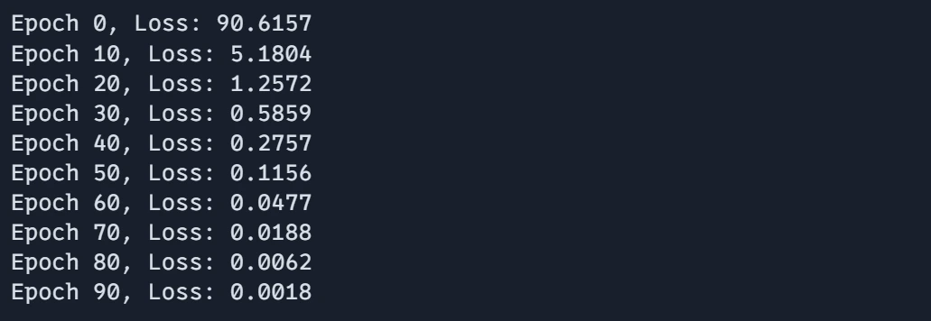
    if epoch % 10 == 0:
        print(f"Epoch {epoch}, Loss: {avg_loss:.4f}")

• Knowledge Technology: Random coaching knowledge (x_data) and corresponding goal (y_data) values are created.    Mannequin and Optimizer Initialization: The mannequin parameters and optimizer state are initialized.
• Coaching Loop: The networks are skilled over a specified variety of epochs, utilizing mini-batch gradient descent.       
• Coaching loops iterate over batches, performing gradient updates utilizing the train_step operate.  The typical loss per epoch is calculated and saved. It prints the epoch quantity and the common loss.

Step8: Plotting the Outcomes

Visualizing the coaching outcomes is vital to understanding the efficiency of our neural community. On this step, we’ll plot the coaching loss over epochs to look at how effectively the mannequin is studying and to determine any potential points within the coaching course of.

# Plot the outcomes
plt.plot(epoch_array, loss_array, label="Coaching Loss")
plt.xlabel("Epoch")
plt.ylabel("Loss")
plt.title("Coaching Loss over Epochs")
plt.legend()
plt.present()

These examples show how JAX combines excessive efficiency with clear, readable code. The useful programming model inspired by JAX makes it simple to compose operations and apply transformations.

Output:

Plot:

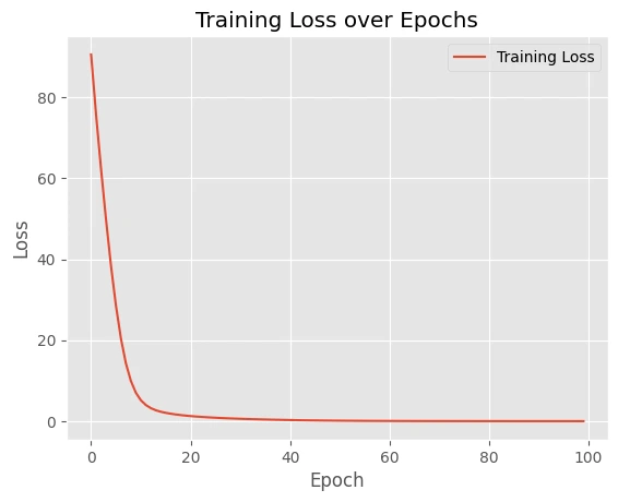
These examples show how JAX combines excessive efficiency with clear, readable code. The useful programming model inspired by JAX makes it simple to compose operations and apply transformations.

Finest Observe and Suggestions

In constructing neural networks, adhering to greatest practices can considerably improve efficiency and maintainability. This part will talk about numerous methods and ideas for optimizing your code and enhancing the general effectivity of your JAX-based fashions.

Efficiency Optimization

Optimizing efficiency is crucial when working with JAX, because it permits us to completely leverage its capabilities. Right here, we’ll discover totally different strategies for enhancing the effectivity of our JAX features, making certain that our fashions run as shortly as attainable with out sacrificing readability.

JIT Compilation Finest Practices

Simply-In-Time (JIT) compilation is among the standout options of JAX, enabling quicker execution by compiling features at runtime. This part will define greatest practices for successfully utilizing JIT compilation, serving to you keep away from widespread pitfalls and maximize the efficiency of your code.

Dangerous Perform

import jax
import jax.numpy as jnp
from jax import jit
from jax import lax


# BAD: Dynamic Python management circulate inside JIT
@jit
def bad_function(x, n):
    for i in vary(n):  # Python loop - can be unrolled
        x = x + 1
    return x
    
    
print("===========================")
# print(bad_function(1, 1000)) # doesn't work
    

This operate makes use of a normal Python loop to iterate n occasions, incrementing the of x by 1 on every iteration. When compiled with jit, JAX unrolls the loop, which will be inefficient, particularly for giant n. This strategy doesn’t absolutely leverage JAX’s capabilities for efficiency.

Good Perform

# GOOD: Use JAX-native operations
@jit
def good_function(x, n):
    return x + n  # Vectorized operation


print("===========================")
print(good_function(1, 1000))

This operate does the identical operation, but it surely makes use of a vectorized operation (x+n) as a substitute of a loop. This strategy is rather more environment friendly as a result of JAX can higher optimize the computation when expressed as a single vectorized operation.

Finest Perform

# BETTER: Use scan for loops


@jit
def best_function(x, n):
    def body_fun(i, val):
        return val + 1

    return lax.fori_loop(0, n, body_fun, x)


print("===========================")
print(best_function(1, 1000))

This strategy makes use of `jax.lax.fori_loop`, which is a JAX-native strategy to implement loops effectively. The `lax.fori_loop` performs the identical increment operation because the earlier operate, but it surely does so utilizing a compiled loop construction. The body_fn operate defines the operation for every iteration, and `lax.fori_loop` executes it from o to n. This technique is extra environment friendly than unrolling loops and is particularly appropriate for circumstances the place the variety of iterations isn’t identified forward of time.

Output:

===========================
===========================
1001
===========================
1001

The code demonstrates totally different approaches to dealing with loops and management circulate inside JAX’s jit-complied features.

Reminiscence Administration

Environment friendly reminiscence administration is essential in any computational framework, particularly when coping with giant datasets or complicated fashions. This part will talk about widespread pitfalls in reminiscence allocation and supply methods for optimizing reminiscence utilization in JAX.

Inefficient Reminiscence Administration

# BAD: Creating giant momentary arrays
@jit
def inefficient_function(x):
    temp1 = jnp.energy(x, 2)  # Momentary array
    temp2 = jnp.sin(temp1)  # One other momentary
    return jnp.sum(temp2)

inefficient_function(x): This operate creates a number of intermediate arrays, temp1, temp1  and eventually the sum of the weather in temp2. Creating these momentary arrays will be inefficient as a result of every step allocates reminiscence and incurs computational overhead, resulting in slower execution and better reminiscence utilization.

Environment friendly Reminiscence Administration

# GOOD: Combining operations
@jit
def efficient_function(x):
    return jnp.sum(jnp.sin(jnp.energy(x, 2)))  # Single operation

This model combines all operations right into a single line of code. It computes the sine of squared parts of x immediately and sums the outcomes. By combining the operation, it avoids creating intermediate arrays, decreasing reminiscence footprints and enhancing efficiency.

Take a look at Code

x = jnp.array([1, 2, 3])
print(x)
print(inefficient_function(x))
print(efficient_function(x))

Output:

[1 2 3]
0.49678695
0.49678695

The environment friendly model leverages JAX’s capacity to optimize the computation graph, making the code quicker and extra memory-efficient by minimizing momentary array creation.

Debugging Methods

Debugging is an important a part of the event course of, particularly in complicated numerical computations. On this part, we’ll talk about efficient debugging methods particular to JAX, enabling you to determine and resolve points shortly.

Utilizing print inside JIT for Debugging

The code reveals strategies for debugging inside JAX, notably when utilizing JIT-compiled features.

import jax.numpy as jnp
from jax import debug


@jit
def debug_function(x):
    # Use debug.print as a substitute of print inside JIT
    debug.print("Form of x: {}", x.form)
    y = jnp.sum(x)
    debug.print("Sum: {}", y)
    return y

# For extra complicated debugging, get away of JIT
def debug_values(x):
    print("Enter:", x)
    end result = debug_function(x)
    print("Output:", end result)
    return end result
    

• debug_function(x): This operate reveals use debug.print() for debugging inside a jit compiled operate. In JAX, common Python print statements are usually not allowed inside JIT attributable to compilation restrictions, so debug.print() is used as a substitute.
• It prints the form of the enter array x utilizing debug.print()
• After computing the sum of the weather of x, it prints the ensuing sum utilizing debug.print()
• Lastly, the operate returns the computed sum y.
• debug_values(x) operate serves as a higher-level debugging strategy, breaking out of the JIT context for extra complicated debugging. It first prints the inputs x utilizing common print assertion. Then calls debug_function(x) to compute the end result and eventually prints the output earlier than returning the outcomes.

Output:

print("===========================")
print(debug_function(jnp.array([1, 2, 3])))
print("===========================")
print(debug_values(jnp.array([1, 2, 3])))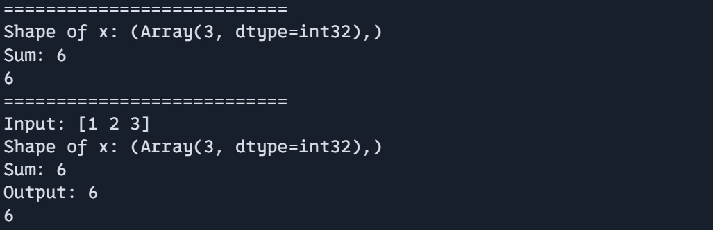

This strategy permits for a mix of in-JIT debugging with debug.print() and extra detailed debugging outdoors of JIT utilizing commonplace Python print statements.

Widespread Patterns and Idioms in JAX

Lastly, we’ll discover widespread patterns and idioms in JAX that may assist streamline your coding course of and enhance effectivity. Familiarizing your self with these practices will help in growing extra sturdy and performant JAX purposes.

System Reminiscence Administration for Processing Giant Datasets

# 1. System Reminiscence Administration
def process_large_data(knowledge):
    # Course of in chunks to handle reminiscence
    chunk_size = 100
    outcomes = []

    for i in vary(0, len(knowledge), chunk_size):
        chunk = knowledge[i : i + chunk_size]
        chunk_result = jit(process_chunk)(chunk)
        outcomes.append(chunk_result)

    return jnp.concatenate(outcomes)


def process_chunk(chunk):
    chunk_temp = jnp.sqrt(chunk)
    return chunk_temp

This operate processes giant datasets in chunks to keep away from overwhelming machine reminiscence.   

It units chunk_size to 100 and iterates over the info increments of the chunk dimension, processing every chunk individually.   

For every chunk, the operate makes use of jit(process_chunk) to JIT-compile the processing operation, which improves efficiency by compiling it forward of time.   

The results of every chunk is concatenated right into a single array utilizing jnp.concatenated(end result) to kind a single record.

Output:

print("===========================")
knowledge = jnp.arange(10000)
print(knowledge.form)

print("===========================")
print(knowledge)

print("===========================")
print(process_large_data(knowledge))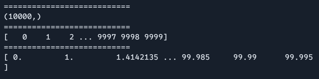

Dealing with Random Seed for Reproducibility and Higher Knowledge Technology

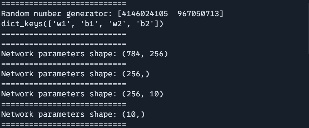
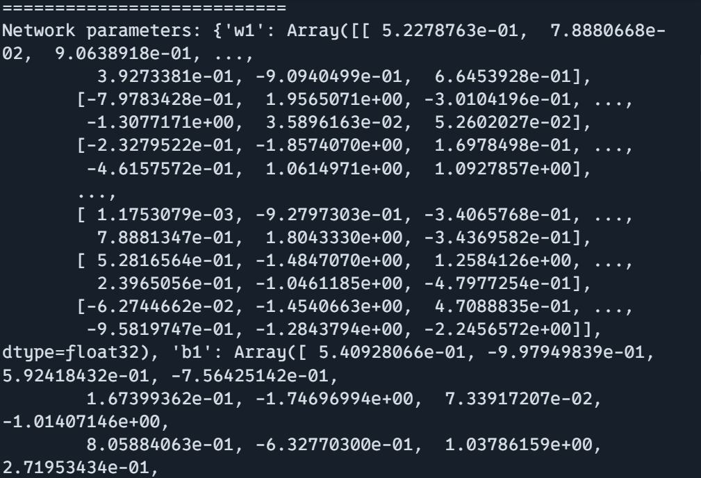
The operate create_traing_state() demonstrates managing random quantity turbines (RNGs) in JAX, which is crucial for reproducibility and constant outcomes.

# 2. Dealing with Random Seeds
def create_training_state(rng):
    # Break up RNG for various makes use of
    rng, init_rng = jax.random.cut up(rng)
    params = init_network(init_rng)

    return params, rng  # Return new RNG for subsequent use
    

It begins with an preliminary RNG (rng) and splits it into two new RNGs utilizing jax.random.cut up(). Break up RNGs carry out totally different duties: `init_rng` initializes community parameters, and the up to date RNG returns for subsequent operations.

The operate returns each the initialized community parameters and the brand new RNG for additional use, making certain correct dealing with of random states throughout totally different steps.

Now take a look at the code utilizing mock knowledge

def init_network(rng):
    # Initialize community parameters
    return {
        "w1": jax.random.regular(rng, (784, 256)),
        "b1": jax.random.regular(rng, (256,)),
        "w2": jax.random.regular(rng, (256, 10)),
        "b2": jax.random.regular(rng, (10,)),
    }


print("===========================")

key = jax.random.PRNGKey(0)
params, rng = create_training_state(key)


print(f"Random quantity generator: {rng}")

print(params.keys())

print("===========================")


print("===========================")
print(f"Community parameters form: {params['w1'].form}")

print("===========================")
print(f"Community parameters form: {params['b1'].form}")
print("===========================")
print(f"Community parameters form: {params['w2'].form}")

print("===========================")
print(f"Community parameters form: {params['b2'].form}")


print("===========================")
print(f"Community parameters: {params}")

Output:

Utilizing Static Arguments in JIT

def g(x, n):
    i = 0
    whereas i < n:
        i += 1
    return x + i


g_jit_correct = jax.jit(g, static_argnames=["n"])
print(g_jit_correct(10, 20))

Output:

30

You should use a static argument if JIT compiles the operate with the identical arguments every time. This may be helpful for the efficiency optimization of JAX features.   

from functools import partial


@partial(jax.jit, static_argnames=["n"])
def g_jit_decorated(x, n):
    i = 0
    whereas i < n:
        i += 1
    return x + i


print(g_jit_decorated(10, 20))

If You need to use static arguments in JIT as a decorator you need to use jit within functools. partial() operate.

Output:

30

Now, we have now realized and dived deep into many thrilling ideas and tips in JAX and total programming model.

What’s Subsequent?

• Experiment with Examples: Attempt to modify the code examples to study extra about JAX.    Construct a small venture for a greater understanding of JAX’s transformations and APIs.    Implement classical Machine Studying algorithms with JAX akin to Logistic Regression, Assist Vector Machine, and extra.
• Discover Superior Subjects: Parallel computing with pmap, Customized JAX transformations,   Integration with different frameworks

All code used on this article is right here

Conclusion

JAX is a robust instrument that gives a variety of capabilities for machine studying, Deep Studying, and scientific computing. Begin with fundamentals, experimenting, and get assist from JAX’s lovely documentation and neighborhood. There are such a lot of issues to study and it’ll not be realized by simply studying others’ code you must do it by yourself. So, begin making a small venture at the moment in JAX. The secret’s to Maintain Going, study on the way in which.

Key Takeaways

• Acquainted NumPY-like interface and APIs make studying JAX simple for newcomers. Most NumPY code works with minimal modifications.
• JAX encourages clear useful programming patterns that result in cleaner, extra maintainable code and upgradation. However If builders need JAX absolutely appropriate with Object Oriented paradigm.
• What makes JAX’s options so highly effective is computerized differentiation and JAX’s JIT compilation, which makes it environment friendly for large-scale knowledge processing.
• JAX excels in scientific computing, optimization, neural networks, simulation, and machine studying which makes developer simple to make use of on their respective venture.

Incessantly Requested Questions

The media proven on this article isn’t owned by Analytics Vidhya and is used on the Creator’s discretion.